Home Science Page Data Stream Momentum Directionals Root Beings The Experiment
Read on to find the extension of many of these principles into the general level of integer.
Let us generalize the above results to include the square root of any positive integer, a.
As before, let X+1 = the square root of a.
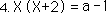
We square both sides of the equation.
We expand our expression, subtract one from both sides of the equation, and then factor out an X.
Dividing by 2+X.
Remembering that X also equals the root minus one from Equation 2.
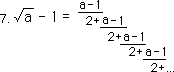
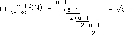
Finally substituting for X on the right side of Equation 5, we arrive at an infinite continued fraction for the root of any integer.
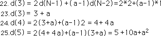
Below are some applications of this equation with some interesting representations. First the square root of 3 as a series of 2s.
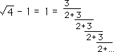
Next the square root of 4 minus one, which equals one, is an infinite continued fraction with lots of 3s and 2s.
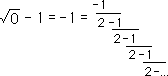
Then the square root of zero minus one or negative one is based upon a lot of 2s and -1s
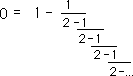
Adding one to both sides, we get an infinite continued fraction for zero, sort of, not quite. It is only borrowing ‘-1’s Infinite Continued Fraction.
More about zero and one a little later.
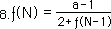
Using a parallel logic to steps 8 thru 15, from our derivation of the series for the square root of two above, we come up with this generalization.
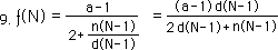
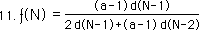
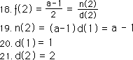
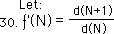
Defining ƒ(N) in terms of a numerator and denominator series, as before. We substitute, then simplify algebraically.
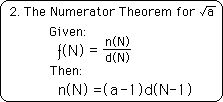
Looking at the numerator of ƒ(N) we see that it determined by the product of a constant, the integer minus one, and the previous element of the denominator series.
We substitute this equality into equation 9.
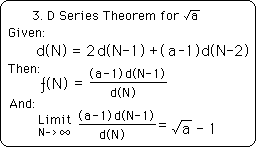
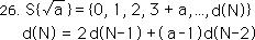
Looking at the denominator of ƒ(N) above, we see that the Nth element of the Denominator Series is defined in terms of the two previous members. Below is the contextual definition of the denominator series that will determine ƒ(N), the F Series for the square root of any positive integer, √a. As before, this is a 2nd order iterative equation.
We notice that ƒ(N) is a function of the Denominator Series. It is the ratio of consecutive members of this series multiplied by the integer minus one, a constant.
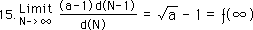
Remembering that the limit of our iterative function is the Root - one, √a - 1, from equations 7 & 8.
Then substituting the results of equation 13, we see that our root is a limit of the ratio of the consecutive members of the denominator series.
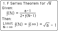
Let us restate our basic theorems in terms of integer square roots. Let us begin with the First Theorem, i.e. the F Series Theorem, for the square root of any positive integer, a.
Notice that this theorem does not contradict the F Series for the √2. It only extends it to more cases. When our integer is 2, the numerator becomes one, (a = 2) -> (a - 1 = 1). turning it into our initial F Series expression, where the numerator was merely one.
Our Second Theorem, the Numerator Theorem, is important because of its ability to neutralize the N Series as a factor in determining the F Series.
Note how once again the original formulation of the Numerator Series is not contradicted, but merely extended.
The Third Theorem, the Denominator Series Theorem, first tells how to generate the D Series. Then it connects the D Series with the F Series and its Limit.
We have another extension of previous results, not a contradiction. These three theorems are primary to the establishment of our Iterative Root Family.
Again these theorems have been tested experimentally via the computer. While the first tests were for the square root of 2, these tests were for a random smattering of integers, each of which tested out accurately. While we might have somehow gotten the square root of 2 to 16 places of accuracy, by chance, it would have been practically impossible to accidentally generate the square roots of a random selection of integers to 16 places. Therefore the experimental verification is greatly strengthened by adding the class of positive integers to the package.
In a similar fashion to the last derivation for the √2, we generate the positive denominator series by using givens, definitions and derivations. Equation 12 is a crucial element in the generation. Equation 12 is the defining equation of the positive Denominator Series. It defines d(N) in terms of the two previous members. It is a contextual series based upon iteration.
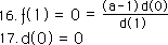
For any iterative series, we need a 'seed' to get the equation going. Because the D Series is derivative from the F Series, we will begin with the F Series. We let the first member of the F Series for √a equal zero, Let ƒ(0) = 0, just as we did before with the F Series for √2. A slight rationale for this assignment is that our F Series is derived by truncating the infinite continued fraction of Equation 7 at regular intervals. The first member is equal to zero because the entire equation is truncated leaving nothing left, zero. Because of this the zeroth member of the denominator series must also be zero. Shown below.
Truncating equation 7 immediately above after the first term, we get the second member of the √a set. From this fact and equation 10 above, we find the first and second members of the denominator series for the √a.
Now that we have two previous elements in the set we can begin generating the rest of the denominator series by employing equation 12.
Finally we can write the positive denominator series for the √a, with the defining equation below. Remember that a function of the ratio of successive members leads to the √a. This is expressed in equation 15.
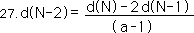
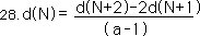
Remembering our great fun with the negative denominator series for √2, remembering our square of solutions, remembering their delicious symmetry, we attempt the same technique with √a. We begin, as we did last time for √2, by solving for d(N-2) in the defining equation immediately above:
Replacing N by N+2, we get the same equation in a different form. Here d(N) is defined by the two successive terms in the series rather than the two previous terms of the series, as in equation 12.
This was the way we got the negative series last time. But this time we have an (a-1) term in the denominator, which fouls everything up. While previously the negative D Series was nearly a mirror opposite of the positive D Series, this definition of the negative Denominator Series leaves us with fractions if a ≠ 2. How inelegant! Further and much more seriously, because of the lack of symmetry in the D Series equation, the negative D Series approaches no limit, and so means nothing.
Many of our theorems are called the First, Second, or Third Theorems because they will extend through all the rational roots. Because of the universality in so many cases, it is tempting to force universality where it doesn’t exist. This is the big problem with pattern recognition and extension. This is why it is so essential to computer test our results. Anyway the point is that our neat little discoveries for the negative D Series for √2, can in no way be generalized, even to the √3. The reason this works so well for √2 is because of the relative symmetry between d(N) and d(N-2) in the D Series equation for √2. The coefficient for both d(N) and d(N-2) is one. Hence the neat little square of positive and negative results shown above in our treatment of √2 only applies to √2 only and to no other root whatsoever. The negative D Series will be forgotten henceforth. It is included here only as an example of where the individual has absolutely no connection with the general.
Thinking metaphorically as always: when we discovered the neat little number square for the iterated expressions for √2, we assumed that the results would easily extend to the general expression. We were thinking of the common spiritual comment that the micro is reflected in the macro and vice versa. We were thinking in common scientific ways about fundamental principles, and building blocks of nature. We were thinking of balanced polarities. While all of these ideas applied to the individual case of √2, they did not extend to one other case. Hence this beauteous positive and negative symmetry is unique and individual to the D Series for √2 alone. Therefore the exploration of general principles would not have revealed the negative series, nor would have the exploration of the properties of the F Series for √2 revealed that this feature could not be extended to the higher levels of generality.
The metaphorical generalization is that general principles do not reveal all the individual characteristics. Further these individual characteristics are only revealed through specific study of the individual. Study of the general only teaches about the general but misses the entire individual structure and personality of specific phenomenon. Thus while the pursuit of general principles is especially important in finding the boundaries of the possible, it is inadequate in revealing all the truly unique specialized characteristics of individual phenomenon. Wherever one looks, personality abounds, which transcends the universal patterns on specific levels. In this case a negative series appears with all its symmetry and polar limits for √2, because of the unique conditions of its expression. But this same negative series with limits exists for no other square root, disappearing immediately into the chaos of no limits for every other number but two.
The major lesson here is to express your individuality. It very well could be unique to the universe, existing only in one's personal world and nowhere else. One's crystalline structure might only appear in conditions specific to oneself but to no one else. Thus in expressing individuality, we are only manifesting our uniqueness in opposition to the general principles of unity that bind the world together. Remember this is not in violation of general principles. It is only an example of specific order and structure, where all else is nearly random chaos. While the universal did not mandate universal chaos or specific order, this is what exists.
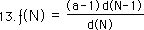
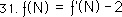
We substitute the expression for d(N) from step 28 into Equation 13 for d(N-1). Doing some basic algebra we get the following simplification.
We let the inverted denominator series equal our inverted square root function.
Substituting back into Equation 29, we get this intriguing equation.
Using the above equation in connection with Equation 15, we get.
Adding one to all parts of the above equation, yields this symmetrical relationship.
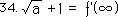
Finally, we get the limit for the inverse function.
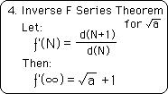
In order to crystallize the discoveries for the inverse F Series, F’, let us state a few of its theorems. First let us formalize the Fourth Theorem, i.e. the inverse F Series theorem for the square root of any positive integer, a.
This theorem defines the inverse F Series, ƒ’, as the inverse ratio of the D Series. It then points out the limit of this series.
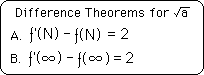
There are also some difference theorems that will also prove useful in the discussions that follow. They are listed below.
Theorem A is a restatement of equation 31 above, while Theorem B is a restatement of Equation 32. Stating these theorems verbally, the difference between the corresponding members of the inverse F Series and the F Series is 2. The difference of their limits is also 2. Both of these difference theorems have been tested upon the computer for a number of integer examples.